Machine learning is increasingly used across industries. ML models make decisions that affect everyday lives, therefore it's important that their predictions are fair, unbiased, and non discriminatory. Accuracy is crucial in many applications that require trust and transparency. In order to ensure fairness in AI, the predictions obtained should be analyzed so that corrective actions shall be taken.
Explaining a model prediction is a low-level mental representation to describe the model's mechanism, while interpreting a model's prediction provides users with a description of what a data point or model output means in context, in a way that humans can understand and trust a model's prediction.

XAI definition

XAI or Explainable AI refers to methods and techniques in the application of artificial intelligence technology such that average humans can understand the results of the solution. It plays a huge part in decision-making and presenting the matter in a transparent way. It contrasts with the concept of black-box in machine learning, where even their designers cannot explain why the AI arrived at a specific decision. When we talk about XAI, we are talking about the impact of the input variables on the output. There are two ways for explaining a model's prediction:

Model specific:

it concerns linear models, decision trees, and generalized additive models, they're called glass-box models because it is easy to trace how the prediction was made. The techniques used are model-specific.

Post-hoc:

They are explanation techniques used after a model has been trained, they treat the model as a BlackBox and they only have the model's inputs and outputs, they are beneficial for boosted trees and neural networks because they're not explainable through model-specific techniques.

SHAP technique:

SHAP, known as shapely additive explanations, is a method based on cooperative game theory to break down a prediction to measure the impact of each feature on the prediction. We will get you started with it via a simple example we'll be running on an xgboost model. We will be using the adult income dataset. It is available on Kaggle via this link.

Installation

Install SHAP using

pip install shap

if it doesn't work try

conda install -c conda-forge shap

shap is supported by many popular algorithms and packages. Seeting up the evironment:

import numpy as np   
import pandas as pd  

# Visualization Libraries
import matplotlib.pyplot as plt
%matplotlib inline

## Machine learning packages
from sklearn.model_selection import train_test_split
import xgboost as xgb

## Model Interpretation package
import shap
shap.initjs()

# Ensuring Reproducibility
SEED = 12345

# Ignoring the warnings
import warnings  
warnings.filterwarnings(action = "ignore")

Dataset

the shap library comes with some commonly used libraries

X,y = shap.datasets.adult()
X_view,y_view = shap.datasets.adult(display=True)
X_view.head()

through this example, you can see that the dataset has attributes such as age, hours of work per week, etc....

Training the model

This step might take few moments

# create a train/test split
X_train, X_valid, y_train, y_valid = train_test_split(X, y, test_size=0.2, random_state=7)

Train the model:

# read in the split dataset into an optimized data structure called Dmatrix required by XGBoost
dtrain = xgb.DMatrix(X_train, label=y_train)
dvalid = xgb.DMatrix(X_valid, label=y_valid)

%%time
# Feed the model the global bias
base_score = np.mean(y_train)
#Set hyperparameters for model training
params = {
   'objective': 'binary:logistic',
   'eval_metric': 'logloss',
   'eta': 0.01,
   'subsample': 0.5,
   'colsample_bytree': 0.8,
   'max_depth': 5,
   'base_score': base_score,
   'seed': SEED
}
# Train using early stopping on the validation dataset.
watchlist = [(dtrain, 'X_train'), (dvalid, 'X_test')]
model = xgb.train(params,        
                       dtrain,                  
                       num_boost_round=5000,                    
                       evals=watchlist,
                       early_stopping_rounds=20,
                       verbose_eval=100)

Calculating the shap values

Use the TreeExplainer class from the shap library to explain the entire dataset containing over 30K samples with over a thousand trees, since we are using a tree-based model.

explainer = shap.TreeExplainer(model=model)
shap_values = explainer.shap_values(X)

Plotting

SHAP force plot

it used to explain one instance of the dataset

classes = {0 : 'False', 1: 'True'}

# ground truth label
y[0]

# Model Prediction
y_pred = [round(value) for value in model.predict(dvalid)]
classes[y_pred[0]]

The observation is False, let's give an insight into how the various features contributed to the model’s prediction for this particular observation.

shap.initjs()
shap.force_plot(explainer.expected_value, shap_values[0,:],X.iloc[0,:])

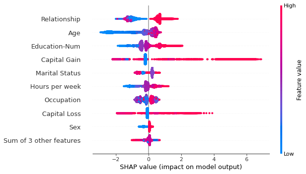
In order to see the impact of the wights distribution in the model, you can use

explainer = shap.Explainer(model)

shap_values = explainer(X)

shap.plots.beeswarm(shap_values)

and it will show something like: